Overview
Empower your data analysis and visualization with a simple yet powerful guide on how to add an X-axis in Google Sheets. This step by step interactive guide helps you to unleash the potential of your charts and graphs by effortlessly labeling and organizing your data along the horizontal axis, creating visually impactful representations that convey insights with clarity and precision.
Who is Google Sheets best suited for?
Google Sheets is best suited for a wide range of professionals, including Financial Analysts, Project Coordinators, and Data Researchers. For example, Financial Analysts can use Google Sheets for budgeting and financial modeling, Project Coordinators can leverage it for tracking project timelines and tasks, and Data Researchers can use it for organizing and analyzing data sets, all benefiting from Google Sheets' collaborative features and powerful data processing tools.
Step by step interactive walkthrough
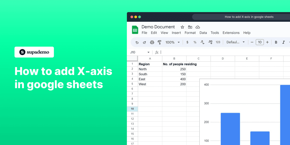
Steps to How to add X-axis in google sheets
1) Navigate to your google sheet document.
2) Double click on the chart to open chart editor.
3) Click on "Setup" 4) Click on the 3 dots icon under the X-axis section.
5) Click on "Add labels"
Common FAQs on Google Sheets
Commonly asked questions about this topic.
How can I create and use a drop-down list in Google Sheets?
How do I merge cells in Google Sheets?
How do I use the QUERY function in Google Sheets?
Enjoyed this interactive product demo?

Justin James
Justin is a growth intern focused on content generation and marketing. He's passionate about making an impact across various startup roles.