Overview
Enhance your financial data presentation in Google Sheets with our guide on formatting currencies. Optimize your workflow by organizing and categorizing monetary values effectively. Improve clarity and streamline data interpretation with easy-to-follow steps for formatting currencies in Google Sheets, ensuring a seamless process to elevate efficiency in financial management.
Who is Google Sheets best suited for?
Google Sheets is best suited for a wide range of professionals, including Accountants, Project Managers, and Marketing Analysts. For example, Accountants can use Google Sheets for financial tracking and reporting, Project Managers can leverage it for planning and monitoring project tasks, and Marketing Analysts can use it for data analysis and campaign performance tracking, all benefiting from Google Sheets’ real-time collaboration and robust data processing capabilities.
How to format currencies in Google Sheets
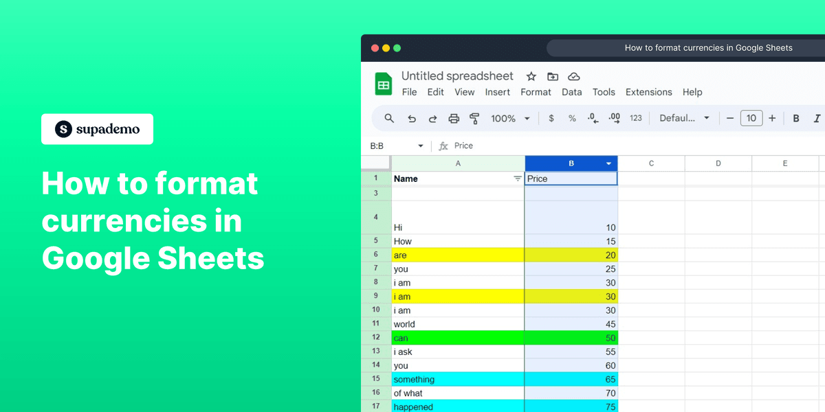
1. Start by selecting the cell or range of cells you want to format.
2. Head to the menu and click the 'Format' option.
3. Proceed by choosing the 'Number' submenu item.
4. Now, select the 'Custom currency' from the available options.
5. Choose the desired currency format, for instance, 'US Dollar'.
6. To finalize, click the 'Apply' button to implement the format.
7. Congratulations on successfully formatting your currency into USD! Review and edit if necessary.
Common FAQs on Google Sheets
Commonly asked questions about this topic.
How do I use conditional formatting in Google Sheets?
How do I freeze rows and columns in Google Sheets?
How do I import data from a website into Google Sheets?
Create your own step-by-step demo
Content Marketer
Nithil is a startup-obsessed operator focused on growth, sales and marketing. He's passionate about wearing different hats across startups to deliver real value.