Overview

Streamline your Google Sheets experience by mastering the art of freezing and unfreezing rows and columns. Elevate your workflow efficiency as you learn the seamless process of anchoring specific rows and columns in place. This comprehensive guide empowers you to enhance clarity and organization within your Google Sheets, ensuring optimal navigation and a more effective approach to data management.

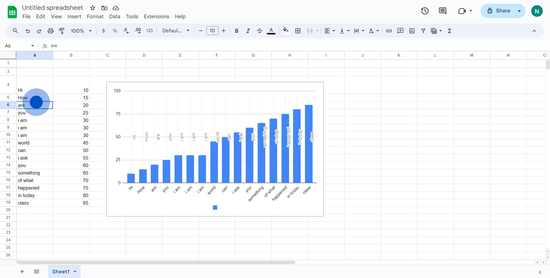
1. Start by selecting all your desired elements.

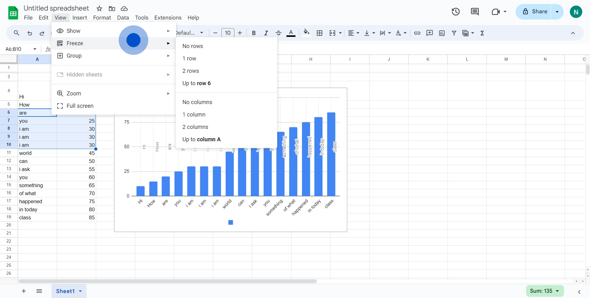
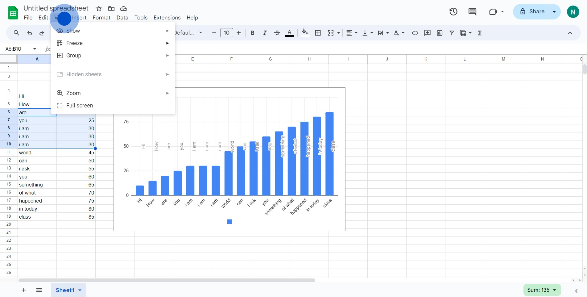
2. Then, go ahead and click on 'View'.

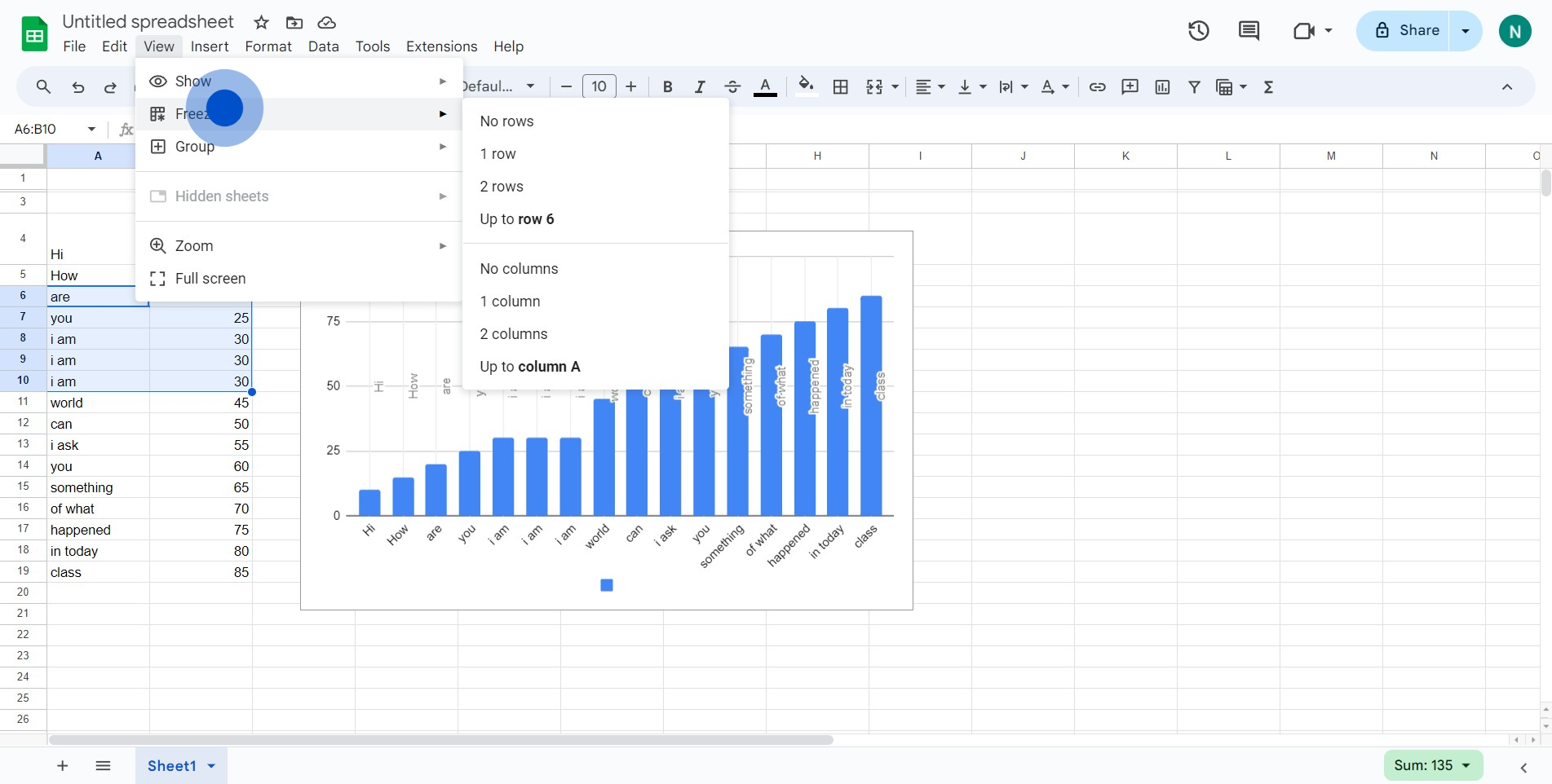
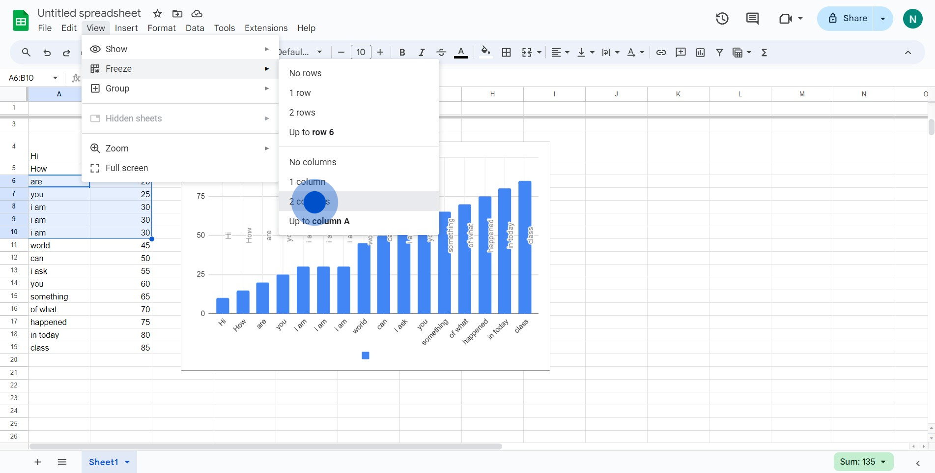
3. Next, find and select the 'Freeze' option.

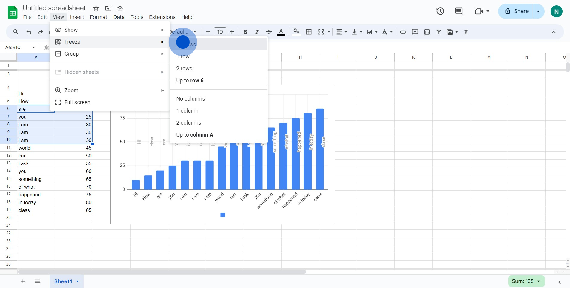
4. Proceed by clicking on 'No rows'.

5. Now, click on 'View' once more.

6. Again, locate and click on 'Freeze'.

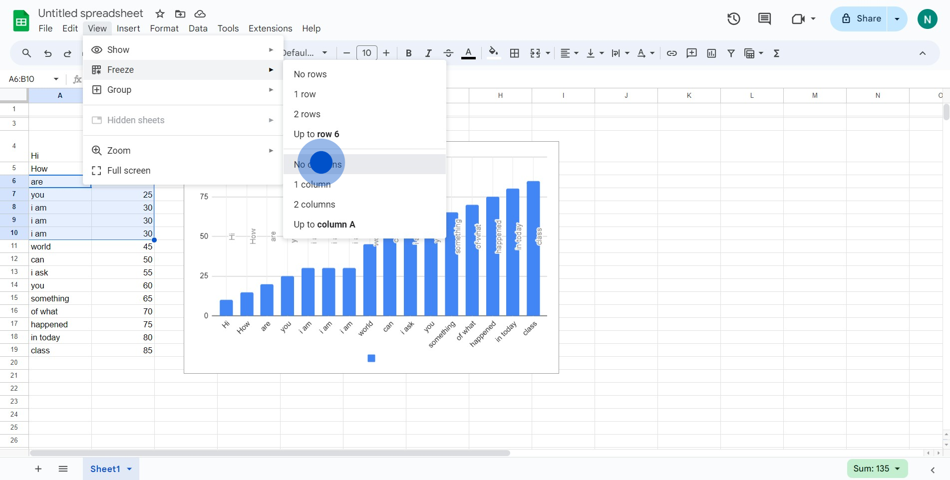
7. Click on 'No columns' to defrost.

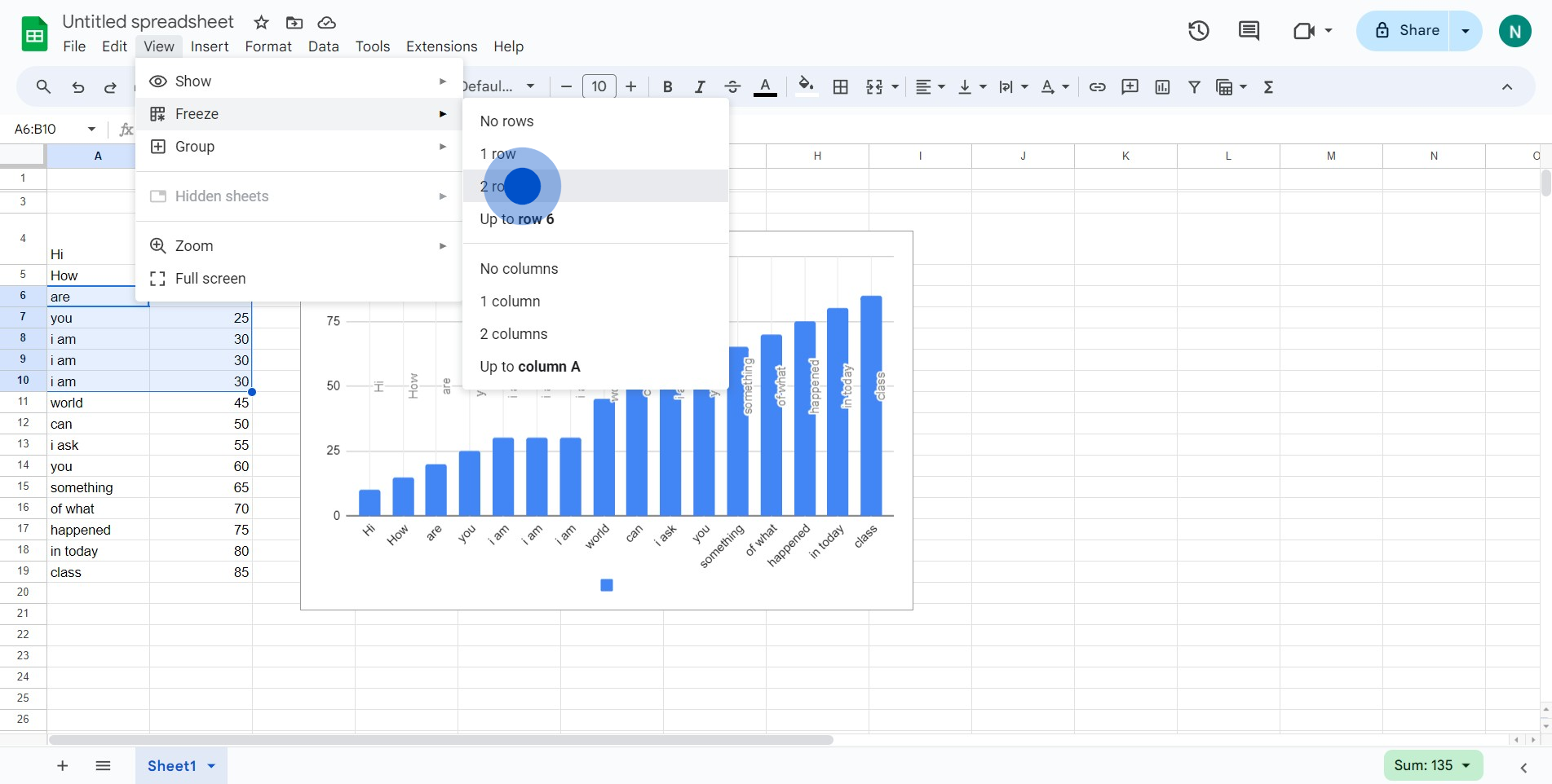
8. Choose '2 rows' to freeze your rows.

9. Lastly, click on '2 columns' to freeze selected columns.

Create your own step-by-step demo

Scale up your training and product adoption with beautiful AI-powered interactive demos and guides. Create your first Supademo in seconds for free.