Overview

Streamline your Google Sheets experience by mastering the art of freezing headings. Enhance workflow organization and ease of navigation by learning how to effectively freeze rows or columns in this comprehensive guide. By following a seamless process, you'll empower yourself to keep essential information readily visible, optimizing efficiency and clarity in your data management within the Google Sheets environment.

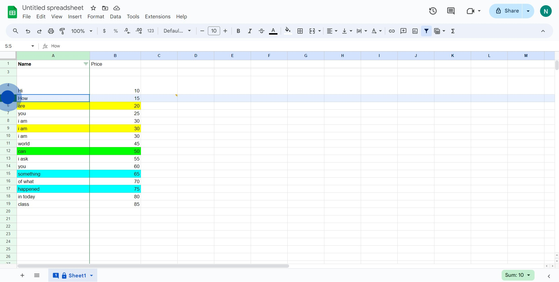
1. Select the row you want to freeze.

2. Now, navigate to the 'View' menu.

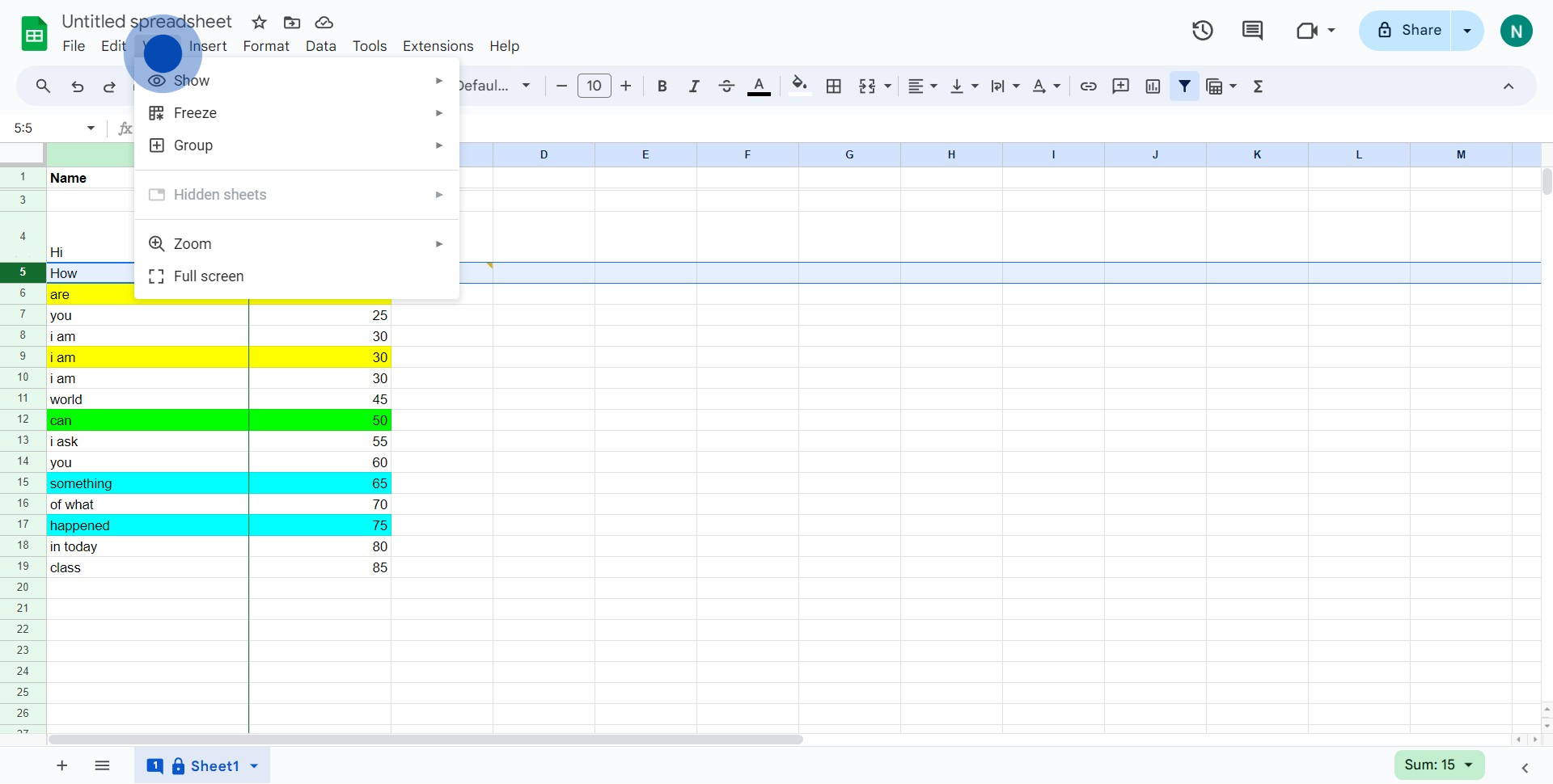
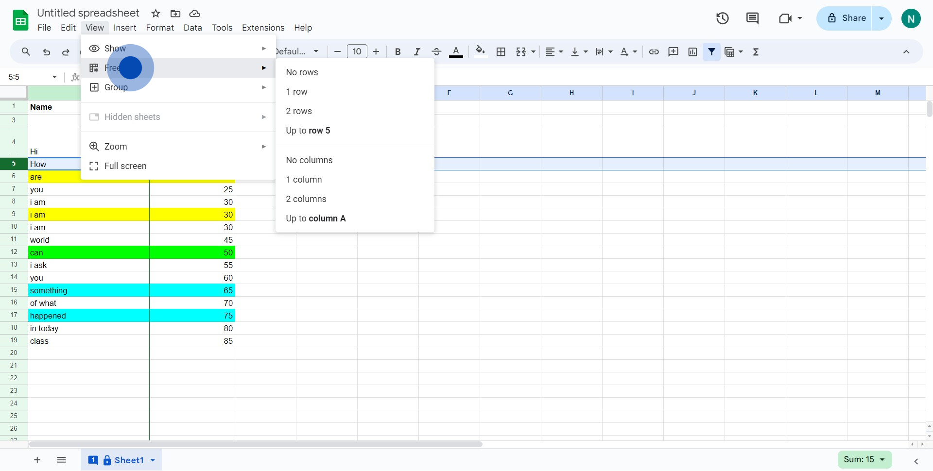
3. Choose the 'Freeze' option from the dropdown list.

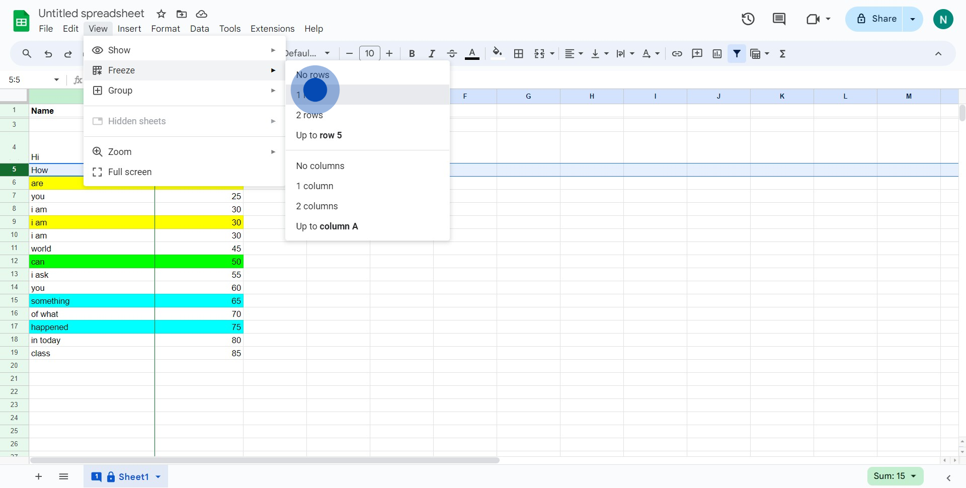
4. Finally, click '1 row' to freeze the selected row.

Create your own step-by-step demo

Scale up your training and product adoption with beautiful AI-powered interactive demos and guides. Create your first Supademo in seconds for free.